Simulating stock prices using GBM

You are expecting the GBM to perform functions it was never set out to perform. By the way, you still have not clarified what exactly you disagree with in provided solutions. You made similar outrageous claims about other models in the past and each time you were schooled and proven wrong...whats new this time?

I know jump diffusion, but it's not the cause/reason here.
 
You are expecting the GBM to perform functions it was never set out to perform.
Elaborate & explain please.

By the way, you still have not clarified what exactly you disagree with in provided solutions. You made similar outrageous claims about other models in the past and each time you were schooled and proven wrong...whats new this time?
BS, I've always been right! Just show me where I was supposedly wrong.
 
GBM by itself is just a base model. You need to add a dynamic risk free rate and simulate the option chain to develop an accurate real word Algo trading system.
GBM.PNG
 
GBM by itself is just a base model. You need to add a dynamic risk free rate and simulate the option chain to develop an accurate real word Algo trading system.View attachment 319811
@Sergio123, it's about GBM itself. The versions I so far tested are all buggy. It much looks like that the well known GBM algorithm(s) in use are all generally buggy in the first place.
And a const r, q, s is ok for me.
 
Last edited:
Here is one
https://people.sc.fsu.edu/~jburkard...on_simulation/brownian_motion_simulation.html


That implementation uses a crude pseudorandom number generator, so you might want to substitute a better one like WELL.
This looks very much professional. I'll study & test it. Thank you very much.

Hmm. I just quickly skimmed over the code, but I'm not sure whether this is really a normal GBM algorithm.
One has to know that there is also just "Brownian Motion" w/o the "Geometric" part, aka ABM, or Arithmetic Brownian Motion.
Need to take more time to study it.

Since there is not a single mentioning of "geometric", then I assume it's not GBM, othweise they would/should explicitly state "geometric". It's just missing.... :-(
 
Last edited:
Since there is not a single mentioning of "geometric", then I assume it's not GBM, othweise they would/should explicitly state "geometric". It's just missing.... :-(

Here is one with geometric in the title.
Geometric Brownian Motion
A stochastic, non-linear process to model asset price
Roman Paolucci

Ifyou have read any of my previous finance articles you’ll notice that in many of them I reference a diffusion or stochastic process known as geometric Brownian motion. I wanted to formally discuss this process in an article entirely dedicated to it which can be seen as an extension to Martingales and Markov Processes. In this article, I want to discuss the purpose and practical applications of this process.

Theoretical applications
The best way to explain geometric Brownian motion is by giving an example where the model itself is required. Consider a portfolio consisting of an option and an offsetting position in the underlying asset relative to the option’s delta.
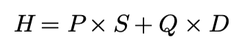
1*_tZMva_9OWRc_0nMJ01XXw.png

Hedge portfolio
Variables:

  • P — Shares of the underlying asset
  • S — Price of the underlying asset
  • Q — Shares of the derivative (option)
  • D — Value of the derivative
  • H — Value of the portfolio
To those of you with more financial experience, or that have read my previous articles, you’ll recognize this as the argument for the Black-Scholes theoretical option pricing model (For a complete derivation and explanation see Deriving the Black-Scholes Model). Note that we can determine the shares (P and Q) of either asset in the portfolio, but we cannot control their values (S and D). In order to determine how to model the option’s price based on this portfolio, we first need to determine a way to model the underlying asset.

Practical applications
Though theoretical applications are important, your primary interest may be as a practitioner. Consider yourself a portfolio manager, based on your team’s market research you are trying to determine the average return of your portfolio. Using geometric Brownian motion in tandem with your research, you can derive various sample paths each asset in your portfolio may follow. This will give you an entire set of statistics associated with portfolio performance from maximum drawdown to expected return. There are uses for geometric Brownian motion in pricing derivatives as well. If you are the underwriter for some exotic you need a way to determine the premium to charge for the risk on your end. One way to accomplish this is to programmatically implement the exotic in a set of sample paths generated by geometric Brownian motion, discounting the average value of the payoff to the present resulting in the fair value of the exotic. For a complete explanation with code see Python for Pricing Exotics or check out the following video.


In the case of either of these applications, we need a way to model the underlying asset.

Mathematical notation
To more accurately model the underlying asset in theory/practice we can modify Brownian motion to include a drift term capturing growth over time and random shocks to that growth.

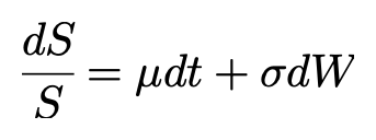
The expression for geometric Brownian motion is actually quite simple…

1*fwTe1fATEQ2RDsZKJvcp2A.png

Geometric Brownian motion
Variables:

  • dS — Change in asset price over the time period
  • S — Asset price for the previous (or initial) period
  • µ — Expected return for the time period or the Drift
  • dt — The change in time (one period of time)
  • σ — Volatility term (a measure of spread)
  • dW — Change in Brownian motion term
Terms:

  • dS/S — Return for a given time period
  • µdt — Expected return for the time period
  • σdW — Random shock to expected return for the time period
Since there is a degree of randomness in this model, every time it's used to simulate an asset’s price it will generate a new path.

Let’s use this equation along with Python to generate a sample path for an asset.

First, we need to build a class that takes in the parameters associated with this model…

Next, we need to create a function that takes a step into the future based on geometric Brownian motion and the size of our time_period all the way into the future until we reach the total_time.

Note: Both time_period and total_time are annualized meaning 1, in either case, refers to 1 year, 1/365 = daily, 1/52 = weekly, 1/12 = monthly.

In the simulate function, we create a new change to the assets price based on geometric Brownian motion and add it to the previous period's price. This change may be positive, negative, or zero and is based on a combination of drift and randomness that is distributed normally with a mean of zero and a variance of dt. This makes sense intuitively, the larger dt (the change in time, or the time period) is the more spread out a collection of samples paths will be. To create a single sample path in the future we can simply create an instance of the 
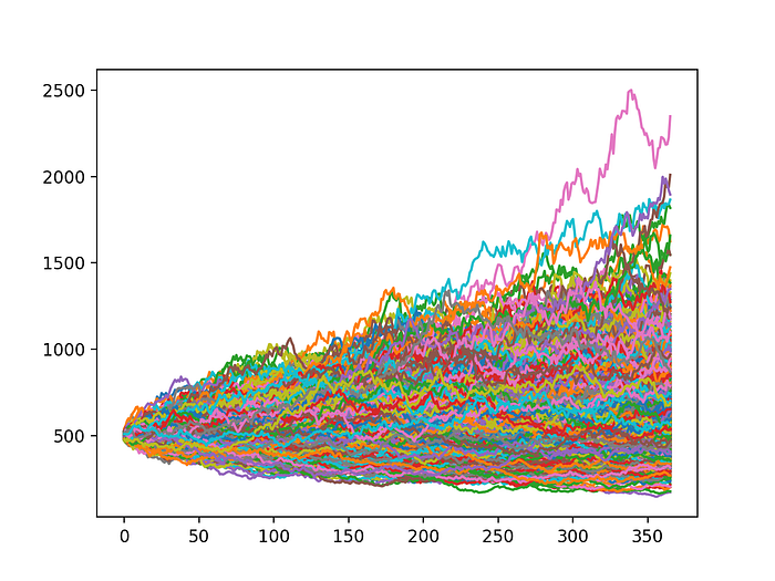
GBM class. However, if we wanted to generate multiple instances of sample paths (and plot it) that follow geometric Brownian motion we can write the following code…

Consequently, we generate 1000 sample paths for the asset based on our parameters which get nicely plotted using matplotlib…

1*RijCTAU0CkEfHKOQ7gcBRg.png

Conclusion
By now you should have a firm grasp on geometric Brownian motion and its theoretical/practical applications. If you are interested in a live explanation with code you can check out the following video…
https://towardsdatascience.com/geometric-brownian-motion-559e25382a55
Code:
import matplotlib.pyplot as plt
import numpy as np
import math


class GBM:

    def simulate(self):
        while(self.total_time > 0):
            dS = self.current_price*self.drift*self.time_period + self.current_price*self.volatility*np.random.normal(0, math.sqrt(self.time_period))
            self.prices.append(self.current_price + dS)
            self.current_price += dS
            self.total_time -= self.time_period

    def __init__(self, initial_price, drift, volatility, time_period, total_time):
        # Initialize fields
        self.initial_price = initial_price
        self.current_price = initial_price
        self.drift = drift
        self.volatility = volatility
        self.time_period = time_period
        self.total_time = total_time
        self.prices = []
        # Simulate the diffusion process
        self.simulate()   # Simulate the diffusion proces

simulations = []
n = 1000
initial_price = 500
drift = .24
volatility = .4
time_period = 1/365 # Daily
total_time = 1

for i in range(0, n):
    simulations.append(GBM(initial_price, drift, volatility, time_period, total_time))

for sim in simulations:
    plt.plot(np.arange(0, len(sim.prices)), sim.prices)

plt.show()
 
@ph1l at al, there are many GBM articles and code on the net, but I need the opinion of experts with hands-on-experience about the quality of the code and algorithm used.
If you are sure & convinced that the algorithm and code is correct then we can focus on it and test further.

Can you math guys check/verify this new code linked by @ph1l with the wikipedia GBM page.
What difference in the algorithm is there, if any?
 
Last edited:
Here is one with geometric in the title.

https://towardsdatascience.com/geometric-brownian-motion-559e25382a55
Code:
import matplotlib.pyplot as plt
import numpy as np
import math


class GBM:

    def simulate(self):
        while(self.total_time > 0):
            dS = self.current_price*self.drift*self.time_period + self.current_price*self.volatility*np.random.normal(0, math.sqrt(self.time_period))
            self.prices.append(self.current_price + dS)
            self.current_price += dS
            self.total_time -= self.time_period

    def __init__(self, initial_price, drift, volatility, time_period, total_time):
        # Initialize fields
        self.initial_price = initial_price
        self.current_price = initial_price
        self.drift = drift
        self.volatility = volatility
        self.time_period = time_period
        self.total_time = total_time
        self.prices = []
        # Simulate the diffusion process
        self.simulate()   # Simulate the diffusion proces

simulations = []
n = 1000
initial_price = 500
drift = .24
volatility = .4
time_period = 1/365 # Daily
total_time = 1

for i in range(0, n):
    simulations.append(GBM(initial_price, drift, volatility, time_period, total_time))

for sim in simulations:
    plt.plot(np.arange(0, len(sim.prices)), sim.prices)

plt.show()
This algorithm & code is interesting as it doesn't use any log(), ln(), e(), or exp() :)
That's very unusual and different from other GBM algos.
I'm now going to test this GBM algo in my test framework...
 
Last edited:
This algorithm & code is interesting as it doesn't use any log(), ln(), e(), or exp() :)
That's very unusual and different from other GBM algos.
I'm now going to test this GBM algo in my test framework...
This algorithm cannot be correct b/c it generates negative stock prices! :) This never ever should happen :)
Code:
Settings used:
  n             = 1000
  initial_price = 500
  drift         = 0.0
  volatility    = 1.5
  time_period   = 0.5       # ie. 2 per year
  total_time    = 1.0       # 1 year

Plot:
pyGBM_wrong.png


Maybe someone inform the author (Roman Paolucci) about this finding so that he maybe can try to fix his algorithm. Link to his article and code is in prev posting.
 
Last edited:
This algorithm cannot be correct b/c it generates negative stock prices! :) This never ever should happen :)
Here's one where the author first codes standard Brownian motion.
https://isquared.digital/blog/2020-04-16-brownian-motion/
Then he uses that for drifted Brownian motion.
https://isquared.digital/blog/2020-05-01-drifted-brownian-motion/
And finally, he uses drifted Brownian motion to implement geometric Brownian motion
https://isquared.digital/blog/2020-05-17-geometric-brownian-motion/#:~:text=Definition of Geometric Brownian Motion&text=This process follows a log,characteristic, they are never negative.
including avoiding negative values.
upload_2023-7-29_8-43-37.png

Code:
import numpy as np
np.random.seed(1234)

def brownian_motion(N, T, h):
    """
    Simulates a Brownian motion
    :param int N : the number of discrete steps
    :param int T: the number of continuous time steps
    :param float h: the variance of the increments
    """
    dt = 1. * T/N  # the normalizing constant
    random_increments = np.random.normal(0.0, 1.0 * h, N)*np.sqrt(dt)  # the epsilon values
    brownian_motion = np.cumsum(random_increments)  # calculate the brownian motion
    brownian_motion = np.insert(brownian_motion, 0, 0.0) # insert the initial condition

    return brownian_motion, random_increments
Code:
import numpy as np

def drifted_brownian_motion(mu, sigma, N, T, seed=42):
    """Simulates a Brownian Motion with drift.

    :param float mu: drift coefficient
    :param float sigma: volatility coefficient
    :param int N : number of discrete steps
    :param int T: number of continuous time steps
    :param int seed: initial seed of the random generator
    :returns list: drifted Brownian motion
    """
    # set the seed
    np.random.seed(seed)
    # standard brownian motion
    W, _ = brownian_motion(N, T ,1.0)
    # the normalizing constant
    dt = 1. * T/N
    # generate the time steps
    time_steps = np.linspace(0.0, N*dt, N+1)
    # calculate the Brownian Motion with drift
    X = mu * time_steps + sigma * W
    return X
Code:
def geometric_brownian_motion(G0, mu, sigma, N, T):
    """Simulates a Geometric Brownian Motion.

    :param float G0: initial value
    :param float mu: drift coefficient
    :param float sigma: diffusion coefficient
    :param int N: number of discrete steps
    :param int T: number of continuous time steps
    :return list: the geometric Brownian Motion
    """
    # the normalizing constant
    dt = 1. * T/N
    # standard brownian motion
    W, _ = brownian_motion(N, T ,1.0)
    # generate the time steps
    time_steps = np.linspace(0.0, N*dt, N+1)

    # calculate the geometric brownian motion
    G = G0 * np.exp(mu * time_steps + sigma * W)
    # replace the initial value
    G[0] = G0

    return G
gbm_monte_carlo.gif
 
Last edited:
Back
Top