
Thank you for spending time to write such a long response to my questions.The math and assumptions are critical when working with utility functions like the Kelly Criterion, but I think I can answer your questions by walking through some plots. Take a look at this Wikipedia link on risk aversion. Go the section labeled 'Example' (or, just see the images I've pasted below). You'll see 3 utility function plots there: risk-averse, risk-neutral, and risk-affine (i.e., risk seeking).
Let's walk through these curves. To be clear, I don't know what utility functions are used in these plots. This is for illustrative purposes. Let's assume the first plot is logarithmic utility (i.e. 'Kelly'). With a logarithm we get decreasing marginal utility. Note in the plot that the slope is steep for small values of W and less steep for larger values. In wealth terms, we can say that our preference for the next dollar of wealth diminishes as our wealth increases - that's built into Kelly. Loosely speaking, because this curve turns inward and down, we call it 'concave'. In contrast, the risk-affine plot turns outward and up - we call that 'convex'.
Let's take a quick look at the other two plots. The risk neutral plot has a constant slope. A bettor with risk neutral utility is indifferent to an uncertain bet and receiving cash. This bettor seeks to earn the expected value of the bet and doesn't require a risk premium (RP). Fractional kelly betting, relative to full Kelly, is increasing risk aversion. For a visual, consider the risk-averse and risk-neutral curves on the same plot. Increasing the risk aversion parameter (smaller Kelly fraction) would reduce the curvature of the risk-averse utility curve. As an exercise, look at the risk-averse plot and see if it makes sense that as risk aversion increases (smaller Kelly fraction), a greater risk premium is required as U(E(W)) increases.
The risk affine plot has an increasing slope. This represents increasing marginal utility. In wealth terms, we can say that our preference for the next dollar of wealth increases as our wealth increases.
Now, let's go back to what I mentioned about widening stop-loss targets and 'scaling in'. Here's what I was thinking... Consider the risk-averse and risk-affine curves on the same plot. Pick a fixed point on the y-axis; call that your trade entry point. As you move below that point the utility loss is smaller for the risk-affine curve. As you move above that point the utility gain is greater for the risk-affine curve. Building on that observation, we could say that the risk-affine bettor gains more utility (relative to the risk-averse bettor) from scaling-in (adding to a winning position) and loses less utility from adding to a losing position. It was in that sense that I commented that adding to a losing position/widening a stop-loss, or adding to a winning position is more consistent with risk-affine utility than risk-aversion. [For a famous example of a bettor with risk-affine characteristics read the story of Jesse Livermore in "Reminiscences of a Stock Operator".]
Regarding your individual trade, if Kelly seems to be working for you in the way that you'd expect that's great. The assumptions of Optimal f aren't as restrictive though.
N.B. Disclaimer: I'm not an expert on Kelly betting, but I've done a decent amount of reading on the topic. So, I'm not representing my understanding as the absolute truth on this. For anyone who is an expert or disagrees, we'd love to hear from you.
risk-averse:
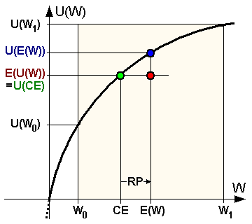
risk-neutral:

risk-affine:

https://en.wikipedia.org/wiki/Risk_aversion
I do have the following comments: Perhaps the three utility functions, instead of describing the risk preference of the better, could instead describe the three different types of system the better bets on?
1. The concave utility function represents a betting system with lots of randomness like stocks/options/blackjack... Because the outcome is governed by randomness, if you bet too big, you are always at the risk of losing it all due to the random nature of the outcome. So, you bet less than optimum?
2. The linear utility function represents a betting system with non random payoff where input and output are known and definitive. If your bet is selling widgets, your payoff depends solely on the number you sell. So, you bet the farm.
3. The convex function represent a betting system where the more you bet the higher your payoff. If your bet is like starting a social media business where the more people you sign up the more your return is. In that case, you want to bet more and more on it as the payoff escalates. So you bet more than the farm, and then some (e.g. starting and running Uber and Lyft).
