
Kelly Criterion & Risk Of Ruin As Risk Management Tool

The math and assumptions are critical when working with utility functions like the Kelly Criterion, but I think I can answer your questions by walking through some plots. Take a look at this Wikipedia link on risk aversion. Go the section labeled 'Example' (or, just see the images I've pasted below). You'll see 3 utility function plots there: risk-averse, risk-neutral, and risk-affine (i.e., risk seeking).

Let's walk through these curves. To be clear, I don't know what utility functions are used in these plots. This is for illustrative purposes. Let's assume the first plot is logarithmic utility (i.e. 'Kelly'). With a logarithm we get decreasing marginal utility. Note in the plot that the slope is steep for small values of W and less steep for larger values. In wealth terms, we can say that our preference for the next dollar of wealth diminishes as our wealth increases - that's built into Kelly. Loosely speaking, because this curve turns inward and down, we call it 'concave'. In contrast, the risk-affine plot turns outward and up - we call that 'convex'.

Let's take a quick look at the other two plots. The risk neutral plot has a constant slope. A bettor with risk neutral utility is indifferent to an uncertain bet and receiving cash. This bettor seeks to earn the expected value of the bet and doesn't require a risk premium (RP). Fractional kelly betting, relative to full Kelly, is increasing risk aversion. For a visual, consider the risk-averse and risk-neutral curves on the same plot. Increasing the risk aversion parameter (smaller Kelly fraction) would reduce the curvature of the risk-averse utility curve. As an exercise, look at the risk-averse plot and see if it makes sense that as risk aversion increases (smaller Kelly fraction), a greater risk premium is required as U(E(W)) increases.

The risk affine plot has an increasing slope. This represents increasing marginal utility. In wealth terms, we can say that our preference for the next dollar of wealth increases as our wealth increases.

Now, let's go back to what I mentioned about widening stop-loss targets and 'scaling in'. Here's what I was thinking... Consider the risk-averse and risk-affine curves on the same plot. Pick a fixed point on the y-axis; call that your trade entry point. As you move below that point the utility loss is smaller for the risk-affine curve. As you move above that point the utility gain is greater for the risk-affine curve. Building on that observation, we could say that the risk-affine bettor gains more utility (relative to the risk-averse bettor) from scaling-in (adding to a winning position) and loses less utility from adding to a losing position. It was in that sense that I commented that adding to a losing position/widening a stop-loss, or adding to a winning position is more consistent with risk-affine utility than risk-aversion. [For a famous example of a bettor with risk-affine characteristics read the story of Jesse Livermore in "Reminiscences of a Stock Operator".]

Regarding your individual trade, if Kelly seems to be working for you in the way that you'd expect that's great. The assumptions of Optimal f aren't as restrictive though.

N.B. Disclaimer: I'm not an expert on Kelly betting, but I've done a decent amount of reading on the topic. So, I'm not representing my understanding as the absolute truth on this. For anyone who is an expert or disagrees, we'd love to hear from you.

risk-averse:
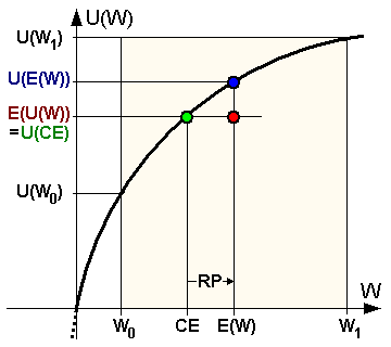
Riskpremium1.png


risk-neutral:
Riskpremium2.png


risk-affine:
Riskpremium3.png


https://en.wikipedia.org/wiki/Risk_aversion
Thank you for spending time to write such a long response to my questions.

I do have the following comments: Perhaps the three utility functions, instead of describing the risk preference of the better, could instead describe the three different types of system the better bets on?

1. The concave utility function represents a betting system with lots of randomness like stocks/options/blackjack... Because the outcome is governed by randomness, if you bet too big, you are always at the risk of losing it all due to the random nature of the outcome. So, you bet less than optimum?

2. The linear utility function represents a betting system with non random payoff where input and output are known and definitive. If your bet is selling widgets, your payoff depends solely on the number you sell. So, you bet the farm.

3. The convex function represent a betting system where the more you bet the higher your payoff. If your bet is like starting a social media business where the more people you sign up the more your return is. In that case, you want to bet more and more on it as the payoff escalates. So you bet more than the farm, and then some (e.g. starting and running Uber and Lyft).
 
Anyone uses Kelly Criterion?

Yes - I use my version of it modified for trading equities & ETFs as opposed to gambling which it was intended for. Max position size is 20% of capital (no margin loans!). I break each position into 4 separate trades of 5% of capital - layering in - adding only to winners. This keeps my loses much smaller than my winners and still allows for the equity curve to have stellar winning years and small draw downs on losing ones (<7%). My risk per trade is just under 1% of capital.
Belt and Suspenders. Nice.
 
Thank you for spending time to write such a long response to my questions.

I do have the following comments: Perhaps the three utility functions, instead of describing the risk preference of the better, could instead describe the three different types of system the better bets on?

1. The concave utility function represents a betting system with lots of randomness like stocks/options/blackjack... Because the outcome is governed by randomness, if you bet too big, you are always at the risk of losing it all due to the random nature of the outcome. So, you bet less than optimum?

2. The linear utility function represents a betting system with non random payoff where input and output are known and definitive. If your bet is selling widgets, your payoff depends solely on the number you sell. So, you bet the farm.

3. The convex function represent a betting system where the more you bet the higher your payoff. If your bet is like starting a social media business where the more people you sign up the more your return is. In that case, you want to bet more and more on it as the payoff escalates. So you bet more than the farm, and then some (e.g. starting and running Uber and Lyft).

You're welcome. Regarding your examples, think of utility (e.g. Kelly) as _your_ risk preference. The examples you've described are _your_ risk preferences for the 3 cases. A typical casino game fits with risk-affine utility. You already know the house has an edge but that's not stopping you from going there. Your example of a social media business is an interesting one. That's consistent with VC firms making subsequent investments in the social media firm at ever-higher valuations. But VC firms definitely seek to earn a risk premium. At the very least, the VC likely has a risk budget constraint.
 
Last edited:
"Increasing the risk aversion parameter (smaller Kelly fraction) would reduce the curvature of the risk-averse utility curve." My apologies, this sentence is incorrect. This would _increase_ the curvature, not reduce. That is, it would increase the concavity.
 
"Increasing the risk aversion parameter (smaller Kelly fraction) would reduce the curvature of the risk-averse utility curve." My apologies, this sentence is incorrect. This would _increase_ the curvature, not reduce. That is, it would increase the concavity.
I think your original statement is more correct. With < 1/2 Kelly you stays at the more linear, less concave part of the curve:
 
I think your original statement is more correct. With < 1/2 Kelly you stays at the more linear, less concave part of the curve:
My choice of words wasn't helping.
Sorry, I've made this more confusing than it needs to be. Let's start with an image. Looking at the previous plot labeled 'risk-averse', think of the bottom right part of the utility curve as anchored at the origin and the upper right part being bent downward. This represents an increase in curvature and an increase in risk aversion. Now, let's formalize this a bit:
The coefficient of relative risk aversion (RRA) is defined as - u"(w)/u'(w). The Kelly utility function is a log utility function E[log(w)]. Fortumately, the RRA for log utility is rather simple, 1/w. We call this 'fractional Kelly'. Now you know where that Kelly fraction comes from :)
 
My choice of words wasn't helping.

Sorry, I've made this more confusing than it needs to be. Let's start with an image. Looking at the previous plot labeled 'risk-averse', think of the bottom right part of the utility curve as anchored at the origin and the upper right part being bent downward. This represents an increase in curvature and an increase in risk aversion. Now, let's formalize this a bit:
The coefficient of relative risk aversion (RRA) is defined as - u"(w)/u'(w). The Kelly utility function is a log utility function E[log(w)]. Fortumately, the RRA for log utility is rather simple, 1/w. We call this 'fractional Kelly'. Now you know where that Kelly fraction comes from :)
Thanks.
 
The Kelly Criterion is just a postulate. Kelly (and Graham as well as Shannon, both of who signed off on the paper) solved for this supposed asymptotic growth-optimal fraction in the 1956 Bell Labs paper, despite the fact that they thought they did solve for it. Actually, they solved for something else. They deluded themselves as they were solving for a subset of problems, the answer to which equaled the asymptotic growth optimal fraction in the narrow cases they were concerned with! Yet people accepted it as fact and still mistakenly do.

The first one to solve for the asymptotic growth optimal fraction was Thorp with his "Kelly Formulas," closed-end formulas for solving for the asymptotic growth-optimal fraction for binomially-distributed outcomes.

The Optimal f formula I put forth in the late 1980s does solve for the asymptotic growth-optimal fraction, for one or more simultaneous propositions (portfolio components/systems/markets). But it too is asymptotic, that is, it is a fraction approached (albeit very quickly) as the number of trials/trades/holding periods increases.

Consider however a game with a positive expectation where you wat to determine the expected growth optimal fraction, but you are quitting after only one play? In such cases, the expected growth optimal fraction, the Optimal f value is 1, or risk 100% to maximize your expected growth after one play.

It's actually a little more complicated than this. Assume a p=.1 to win 10 units and q=.9 to lose 1 unit. Though there is a positive expectation, it is a game you should not play if you are going to quit after one play. Similarly, if we have a negative expectation game with p=.9 to win 1 unit and q=.9 to lose 10 units, and you wish to maximize your expected growth, quitting after one play, your Optimal f = 1, or risk it all on the one play. The Kelly Criterion, even Thorp's Kelly formulas for these binomial outcomes give you entirely different (and incorrect) results.

I refer you to my paper on this at https://papers.ssrn.com/sol3/papers.cfm?abstract_id=2577782

This will give you what the expected growth optimal fraction(s) are for one or more simultaneous propositions, for 1 to infinitely many trials.Further, there are other considerations, such as the fact the there is a cost of funds involved (trades don't transpire instantaneously in most cases), etc.

Anyone who has used "Kelly" with success has been using something that is mathematically incorrect, and the success may in many cases be attributable to luck (you cannot determine an expected growth optimal fraction for most capital market situations with any of what has been referred to as "Kelly," nor can you even apply it, correctly mathematically to the game of blackjack, and favorable results garnered from such were done so with grossly inaccurate calculations).

Finally, all of this assumes your criterion in trading is to be expected growth-optimal, all else (including drawdown or other risk measures) be damned. This is ok provided that really is your criterion.

Since the actual Optimal f value (or value sets) exit between the bookends of 0 and 1, there are other points of geometrical interest within that manifold. Further, everyone in every assumed proposition or set of propositions exists within that manifold,unwittingly in most cases, and are covering paths through it, unwittingly again in most cases.They are paying the consequence and reaping the benefits in terms of performance characteristics that these various points of geometric consequence (aside form the peak, the Optimal f points) imbue. In fact, various points and paths in this manifold can be constructed to satisfy ant trading criteria. It really is not very complicated -- I'm not trying to sell anything, razzle-dazzle anyone, but rather to edify this area that is always misunderstood.

so what you propose the to use ?
 
I run several monte carlo simulations with for a 50/50 system with a 2 to 1 payoff (2 gain or 1 loss). 5000 trades each for 34 trials. With full-kelly the avg max DD -99.4% and it reached that DD in almost every trial and when it didn't, it got close (-98%, etc)
With half-kelly the avg max DD was -89% in each of the trials and it reached that (or gotten close) in almost every trial.
My point is that it seems counter intuitive that risking half as much would still yield DDs that are similar to the full thing. -85%+ DD is quite typical in half kelly system betting and I wasn't aware of that. Advocators of half kelly betting never bring that up

did you check runs for lower than 1/2 ?
 
Back
Top