Yeah, I figured it out as it didn't make any sense otherwise. But I have to say I'm disappointed. Below is equity of your system vs sma260. I thought, low pass filter will beat the crap out of sma.Quote from jcl:
No, the asset price - they are filled from *Data.
You are using an out of date browser. It may not display this or other websites correctly.
You should upgrade or use an alternative browser.
You should upgrade or use an alternative browser.
Automated Trading Course - Part 2: Writing Strategies
- Thread starter jcl
- Start date
This would be the result of this system with SMA 260:
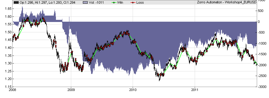
An SMA with a fixed period can normally not generate a consistent profitable trend signal. You can indeed create a profitable system even with a SMA, but then you have to adapt the period to the asset and market situation. How to do such an adaption will be the subject of the next lesson.
An SMA with a fixed period can normally not generate a consistent profitable trend signal. You can indeed create a profitable system even with a SMA, but then you have to adapt the period to the asset and market situation. How to do such an adaption will be the subject of the next lesson.
This has nothing to do with the market. You can not use the same time periods for hourly and daily bars, as the system would then trigger only 3 trades with daily silver. A test with only 3 trades in 4 years is meaningless. You need about 100 trades for a useful test result.
When you test with a reasonable number of trades, such as Lowpass 1000 vs. SMA 260 with hourly silver, you get 52% profit for Lowpass, and 8% loss for SMA 260. Just try it.
You can certainly construct a special system where a SMA with a special time period is more profitable than a Lowpass function. But in most systems and markets that I've tested, the Lowpass filter generates not only more profit, it is normally also more robust, meaning the profit is less dependent from its time period parameter.
In the next lesson we'll look into how to optimize a strategy and use better test methods. Bob got a new trade idea:
Bob: Last month I ran into Warren Buffett and asked him for a trading advice. That's what he said: 'Be greedy when others are fearful'.
Alice: Interesting. And what does it mean?
Bob: He didn't tell, but went away. But I think he wants me to go against the trend.
Alice: Isn't that just the opposite of your last strategy?
Bob: You got it. I need you to automatize this. I now buy long when prices moved down very much, and go short when they moved up very much.
Alice: How much is very much?
Bob: Depends on the market.
Alice: I should have known.
Bob: Well, prices often move up and down in cycles. Problem is, cycles are sometimes not easy to see in the price curve. You must find the main price cycle and check if the price comes close to its top or bottom. Then you know the right moment to buy or sell.
Alice: I can use a frequency analysis function to find the dominant period of the price cycle.
Bob: If you say so.
Alice: Then I only need to find the top and bottom. I use the dominant period to control a highpass filter. This will cut off the trend and all cycles below the dominant period and give me a clean cycle curve.
Bob: Sounds good.
Alice: For finding how close the cycle is to its peaks, I must normalize the curve. For instance with a Fisher transformation. This has the advantage that the curve gets a Gaussian distribution. There are less extrema, and they are relatively sharp and well defined, so we won't get too many false signals.
Bob: Sharp and well defined. I like that.
Alice: Of course it's much more complicated than trend trading. This comes at a higher fee.
Bob: I like that less.
Alice: But I can run a Walk Forward Optimization as an extra.
Bob: Huh? Will that get me more profit?
Alice: Yes. So that you can afford me.
Alice went home and wrote this script (fee: $12,000):
This system looks more complex than the simple trend trading system. Tomorrow we'll go through the code and analyze it.
Bob: Last month I ran into Warren Buffett and asked him for a trading advice. That's what he said: 'Be greedy when others are fearful'.
Alice: Interesting. And what does it mean?
Bob: He didn't tell, but went away. But I think he wants me to go against the trend.
Alice: Isn't that just the opposite of your last strategy?
Bob: You got it. I need you to automatize this. I now buy long when prices moved down very much, and go short when they moved up very much.
Alice: How much is very much?
Bob: Depends on the market.
Alice: I should have known.
Bob: Well, prices often move up and down in cycles. Problem is, cycles are sometimes not easy to see in the price curve. You must find the main price cycle and check if the price comes close to its top or bottom. Then you know the right moment to buy or sell.
Alice: I can use a frequency analysis function to find the dominant period of the price cycle.
Bob: If you say so.
Alice: Then I only need to find the top and bottom. I use the dominant period to control a highpass filter. This will cut off the trend and all cycles below the dominant period and give me a clean cycle curve.
Bob: Sounds good.
Alice: For finding how close the cycle is to its peaks, I must normalize the curve. For instance with a Fisher transformation. This has the advantage that the curve gets a Gaussian distribution. There are less extrema, and they are relatively sharp and well defined, so we won't get too many false signals.
Bob: Sharp and well defined. I like that.
Alice: Of course it's much more complicated than trend trading. This comes at a higher fee.
Bob: I like that less.
Alice: But I can run a Walk Forward Optimization as an extra.
Bob: Huh? Will that get me more profit?
Alice: Yes. So that you can afford me.
Alice went home and wrote this script (fee: $12,000):
Code:
function run()
{
  BarPeriod = 240; // 4 hour bars

// calculate the buy/sell signal
  var *Price = series(price());
  var *DomPeriod = series(DominantPeriod(Price,30));
  var LowPeriod = LowPass(DomPeriod,500);
  var *HP = series(HighPass(Price,LowPeriod));
  var *Signal = series(Fisher(HP,500));
  var Threshold = 1.0;
  Stop = 2*ATR(100);

// buy and sell
  if(crossUnder(Signal,-Threshold))
    enterLong();
  else if(crossOver(Signal,Threshold))
    enterShort();

// plot signals and thresholds
  plot("DominantPeriod",LowPeriod,NEW,BLUE);
  plot("Signal",Signal[0],NEW,RED);
  plot("Threshold1",Threshold,0,BLACK);
  plot("Threshold2",-Threshold,0,BLACK);
  PlotWidth = 1000;
  PlotHeight1 = 300;
}
This system looks more complex than the simple trend trading system. Tomorrow we'll go through the code and analyze it.
Quote from jcl:
When you test with a reasonable number of trades, such as Lowpass 1000 vs. SMA 260 with hourly silver, you get 52% profit for Lowpass, and 8% loss for SMA 260. Just try it..
What period? I've tested silver since 2010/05/25 and both sma and low pass make no significant profit.
The period was 2008 to 2011, just the same as for the other tests.
- May I make a suggestion? This course is more about how to convert a trade idea into an automated strategy, rather than discussing SMA vs. lowpass. But you can open another thread for this, maybe in the TA forum. I'll answer there, and we can look into under which circumstances a lowpass filter is better and when a SMA might be better. I also suspect that something might be wrong with your lowpass implementation, because your posted curves of lowpass and SMA results look quite similar, which should normally not be the case. You can test if a frequency filter is implemented correctly by applying it to a sinus curve with varied frequency.
- May I make a suggestion? This course is more about how to convert a trade idea into an automated strategy, rather than discussing SMA vs. lowpass. But you can open another thread for this, maybe in the TA forum. I'll answer there, and we can look into under which circumstances a lowpass filter is better and when a SMA might be better. I also suspect that something might be wrong with your lowpass implementation, because your posted curves of lowpass and SMA results look quite similar, which should normally not be the case. You can test if a frequency filter is implemented correctly by applying it to a sinus curve with varied frequency.
Back to work. Alice had written the following script for a counter trend strategy:
Counter trend trading is affected by market cycles and more sensitive to the bar period than trend trading. Bob has told Alice that bar periods that are in sync with the worldwide markets - such as 4 or 8 hours - are especially profitable with this type of trading. Therefore she has set the bar period to a fixed value of 4 hours, or 240 minutes:
BarPeriod = 240;
The counter trend trade rules are contained in the following lines that calculate the buy/sell signal:
var *Price = series(price());
var *DomPeriod = series(DominantPeriod(Price, 30));
var LowPeriod = LowPass(DomPeriod, 500);
var *HP = series(HighPass(Price, LowPeriod));
var *Signal = series(Fisher(HP, 500));
The first line sets up a price series just as in the last workshop. The next one calculates the dominant period. That's the most significant cycle in a price curve which is normally a superposition of many cycles. If prices would oscillate up and down every two weeks, the dominant period would be 60 - that's the length of two weeks, resp. 10 trade days, counted in 4-hour-bars. Alice uses the DominantPeriod() analysis function with a cutoff period of 30 bars for finding the main price oscillation cycle in the range below 100 bars. The result DomPeriod is a series of dominant periods.
Because the dominant period fluctuates a lot, the next line passes the series through a lowpass filter, just like the price curve of the last workshop. The result is stored in a variable (not a series, thus no '*') LowPeriod that is the lowpass filtered dominant period of the current price curve.
In the next line, a highpass filter is fed with the price curve and its cutoff frequency is set to the dominant period. This removes the trend and all cycles that are lower than the dominant period from the price curve. The HighPass() function is similar to the LowPass function, it just does the opposite, and leaves only high frequencies, i.e. short cycles, in the price curve. The result is a modified price curve that consists mostly of the dominant cycle. It's stored in a new series named HP (for HighPass).
Alice is not finished yet. The HP series is now compressed into a Gaussian distribution by applying the Fisher Transformation. This is an operation used to transform an arbitrary curve into a range where most values are in the middle - around 0 - and only few values are outside the +1...-1 range. For this transformation she calls the Fisher() function. It compresses the last 500 bars from the HP series into the Gaussian distributed Signal series. This method of trading with highpass filters, cycle detectors, and Fisher transform was developed by John Ehlers, an engineer who used signal processing methods for trading.
The next two lines define a new variable Threshold with a value of 1.0, and place a stop loss at an adaptive distance from the price, just as in Alice's trend trading script from some lessons ago. The ATR function is again used to determine the stop loss.
var Threshold = 1.0;
Stop = 2*ATR(100);
Now that the preparation is done, we can start trading:
if(crossUnder(Signal, -Threshold))
enterLong();
else if(crossOver(Signal, Threshold))
enterShort();
When the Signal curve cosses the negative threshold from above - meaning when Signal falls below -1 - the price is supposedly at the bottom of the dominant cycle, so we expect the price to rise and buy long. When the threshold is crossed from below - meaning Signal rises above 1 - the price is at a peak and we buy short. This is just the opposite of what we did in trend trading. For identifying the threshold crossing we're using the crossOver() and crossUnder() functions.
- Obviously, these trade rules are somewhat more complicated than the simple lowpass function of the previous lesson. So Alice needs to see how the various series look, for checking if everything works as supposed. The next line (at the end of the script)
plot("DominantPeriod", LowPeriod, NEW, BLUE);
generates a plot of the LowPeriod variable in a NEW chart window with color BLUE. We can use this function to plot anything into the chart, either in the main chart with the price and equity curve, or below the main chart in a new window. The Signal curve and the upper and lower Threshold are plotted in another new chart window:
plot("Signal", Signal[0], NEW, RED);
plot("Threshold1", Threshold, 0, BLACK);
plot("Threshold2", -Threshold, 0, BLACK);
The first statement plots the Signal[0] value as a red curve (as we remember, adding a [0] to a series name gives its most recent value). The next two statements plot the positive and negative Threshold with two black lines in the same chart window. Note that the plot function always expects a value, not a series - that's why we needed to add the [0] to the Signal name.
PlotWidth = 1000;
PlotHeight1 = 300;
This just sets the width and height of the chart window. Below is the resulting chart. Load the script workshop5_1 and make sure that EUR/USD is selected. Click [Test], then click [Result]:
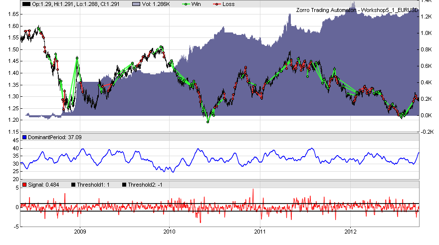
The blue curve in the middle window is the plot of LowPeriod. It moves mostly between 25 and 40 bars, corresponding to a 4..7 days dominant cycle. The bottom window shows the Signal series. The black lines are the thresholds that trigger buy and sell signals when Signal crosses over or under them. Plotting variables and series in the chart greatly helps to understand and improve the trade rules. For examining a part of the chart in details, the StartDate and NumDays variables can be used to limit the number of bars to plot and 'zoom into' a part of the chart.
We can see that the script generates 139% annual return. This is already better than the simple trend trading script from the last workshop; but the equity curve is still not satisfying. Alice has to do more for her fee and improve this strategy further. We'll do that tomorrow.
Code:
function run()
{
  BarPeriod = 240; // 4 hour bars

// calculate the buy/sell signal
  var *Price = series(price());
  var *DomPeriod = series(DominantPeriod(Price,30));
  var LowPeriod = LowPass(DomPeriod,500);
  var *HP = series(HighPass(Price,LowPeriod));
  var *Signal = series(Fisher(HP,500));
  var Threshold = 1.0;
  Stop = 2*ATR(100);

// buy and sell
  if(crossUnder(Signal,-Threshold))
    enterLong();
  else if(crossOver(Signal,Threshold))
    enterShort();

// plot signals and thresholds
  plot("DominantPeriod",LowPeriod,NEW,BLUE);
  plot("Signal",Signal[0],NEW,RED);
  plot("Threshold1",Threshold,0,BLACK);
  plot("Threshold2",-Threshold,0,BLACK);
  PlotWidth = 1000;
  PlotHeight1 = 300;
}
Counter trend trading is affected by market cycles and more sensitive to the bar period than trend trading. Bob has told Alice that bar periods that are in sync with the worldwide markets - such as 4 or 8 hours - are especially profitable with this type of trading. Therefore she has set the bar period to a fixed value of 4 hours, or 240 minutes:
BarPeriod = 240;
The counter trend trade rules are contained in the following lines that calculate the buy/sell signal:
var *Price = series(price());
var *DomPeriod = series(DominantPeriod(Price, 30));
var LowPeriod = LowPass(DomPeriod, 500);
var *HP = series(HighPass(Price, LowPeriod));
var *Signal = series(Fisher(HP, 500));
The first line sets up a price series just as in the last workshop. The next one calculates the dominant period. That's the most significant cycle in a price curve which is normally a superposition of many cycles. If prices would oscillate up and down every two weeks, the dominant period would be 60 - that's the length of two weeks, resp. 10 trade days, counted in 4-hour-bars. Alice uses the DominantPeriod() analysis function with a cutoff period of 30 bars for finding the main price oscillation cycle in the range below 100 bars. The result DomPeriod is a series of dominant periods.
Because the dominant period fluctuates a lot, the next line passes the series through a lowpass filter, just like the price curve of the last workshop. The result is stored in a variable (not a series, thus no '*') LowPeriod that is the lowpass filtered dominant period of the current price curve.
In the next line, a highpass filter is fed with the price curve and its cutoff frequency is set to the dominant period. This removes the trend and all cycles that are lower than the dominant period from the price curve. The HighPass() function is similar to the LowPass function, it just does the opposite, and leaves only high frequencies, i.e. short cycles, in the price curve. The result is a modified price curve that consists mostly of the dominant cycle. It's stored in a new series named HP (for HighPass).
Alice is not finished yet. The HP series is now compressed into a Gaussian distribution by applying the Fisher Transformation. This is an operation used to transform an arbitrary curve into a range where most values are in the middle - around 0 - and only few values are outside the +1...-1 range. For this transformation she calls the Fisher() function. It compresses the last 500 bars from the HP series into the Gaussian distributed Signal series. This method of trading with highpass filters, cycle detectors, and Fisher transform was developed by John Ehlers, an engineer who used signal processing methods for trading.
The next two lines define a new variable Threshold with a value of 1.0, and place a stop loss at an adaptive distance from the price, just as in Alice's trend trading script from some lessons ago. The ATR function is again used to determine the stop loss.
var Threshold = 1.0;
Stop = 2*ATR(100);
Now that the preparation is done, we can start trading:
if(crossUnder(Signal, -Threshold))
enterLong();
else if(crossOver(Signal, Threshold))
enterShort();
When the Signal curve cosses the negative threshold from above - meaning when Signal falls below -1 - the price is supposedly at the bottom of the dominant cycle, so we expect the price to rise and buy long. When the threshold is crossed from below - meaning Signal rises above 1 - the price is at a peak and we buy short. This is just the opposite of what we did in trend trading. For identifying the threshold crossing we're using the crossOver() and crossUnder() functions.
- Obviously, these trade rules are somewhat more complicated than the simple lowpass function of the previous lesson. So Alice needs to see how the various series look, for checking if everything works as supposed. The next line (at the end of the script)
plot("DominantPeriod", LowPeriod, NEW, BLUE);
generates a plot of the LowPeriod variable in a NEW chart window with color BLUE. We can use this function to plot anything into the chart, either in the main chart with the price and equity curve, or below the main chart in a new window. The Signal curve and the upper and lower Threshold are plotted in another new chart window:
plot("Signal", Signal[0], NEW, RED);
plot("Threshold1", Threshold, 0, BLACK);
plot("Threshold2", -Threshold, 0, BLACK);
The first statement plots the Signal[0] value as a red curve (as we remember, adding a [0] to a series name gives its most recent value). The next two statements plot the positive and negative Threshold with two black lines in the same chart window. Note that the plot function always expects a value, not a series - that's why we needed to add the [0] to the Signal name.
PlotWidth = 1000;
PlotHeight1 = 300;
This just sets the width and height of the chart window. Below is the resulting chart. Load the script workshop5_1 and make sure that EUR/USD is selected. Click [Test], then click [Result]:
The blue curve in the middle window is the plot of LowPeriod. It moves mostly between 25 and 40 bars, corresponding to a 4..7 days dominant cycle. The bottom window shows the Signal series. The black lines are the thresholds that trigger buy and sell signals when Signal crosses over or under them. Plotting variables and series in the chart greatly helps to understand and improve the trade rules. For examining a part of the chart in details, the StartDate and NumDays variables can be used to limit the number of bars to plot and 'zoom into' a part of the chart.
We can see that the script generates 139% annual return. This is already better than the simple trend trading script from the last workshop; but the equity curve is still not satisfying. Alice has to do more for her fee and improve this strategy further. We'll do that tomorrow.
jcl,
Are the functions you referenced (fisher, lowpass, highpass, dominantcycle) already included with Zorro?
If so, are they open source?
Are the functions you referenced (fisher, lowpass, highpass, dominantcycle) already included with Zorro?
If so, are they open source?