Hi,
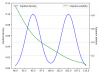
I'm interested in modelling the volatility skew of a stock with a bimodal outcome. I found this blogpost and want to reproduce its findings. I am struggling with the implied volatility-part.
I know that the probability density function is equal to
$f(S) = \sum^n_{i=1}p_i\frac{1}{\sqrt{2\pi}\sigma_i}exp\{-\frac{(S-\mu_i)^2}{2\sigma_i^2}\}$
I also know that the price of a call can be defined as
$C=e^{-rT}\int_0^\infty(S-K)^+p(S)dS$
My plotted implied volatility looks different than the authors. What am I doing wrong? My methodology
- obtain the PDF
- get the price of the call using this PDF
- get IV based on price of the call
I attached my Python code for clarity:
import numpy as np
import scipy.stats as ss
import matplotlib.pyplot as plt
from black_scholes import *
from typing import Union
def f(mu: float, sigma: float, x: np.ndarray) -> np.ndarray:
return np.exp((-1 * (x - mu) ** 2) / (2 * sigma ** 2)) / (np.sqrt(2 * np.pi) * sigma)
def call(r: float, T: float, S: np.ndarray, K: Union[int, float], pdf: np.ndarray) -> float:
inner = np.zeros_like(S)
itm = S > K
inner[itm] = S[itm] - K
return np.exp(-r * T) * np.sum(inner * pdf)
def price(S, K, T, r, sigma):
# https://www.aaronschlegel.me/black-scholes-formula-python.html
d1 = (np.log(S / K) + (r + 0.5 * sigma ** 2) * T) / (sigma * np.sqrt(T))
d2 = (np.log(S / K) + (r - 0.5 * sigma ** 2) * T) / (sigma * np.sqrt(T))
return S * ss.norm.cdf(d1, 0.0, 1.0) - K * np.exp(-r * T) * ss.norm.cdf(d2, 0.0, 1.0)
def vega(S, K, T, r, sigma):
d1 = (np.log(S / K) + (r + 0.5 * sigma ** 2) * T) / (sigma * np.sqrt(T))
return S * ss.norm.pdf(d1) * np.sqrt(T)
def iv(c, S, K, T, r):
MAX_ITERATIONS = 200
PRECISION = 1.0e-5
sigma = 0.25
for _ in range(MAX_ITERATIONS):
p = price(S, K, T, r, sigma)
v = vega(S, K, T, r, sigma)
diff = c - p
if abs(diff) < PRECISION:
return sigma
sigma = sigma + diff / v
return sigma
S = 100
n = 2
p_up = 0.5
p_down = 1 - p_up
mu_up = 105
sigma_up = 2
mu_down = 95
sigma_down = 2
T = np.sqrt(7 / 255)
r = 0
if __name__ == "__main__":
dx = 0.5
xs = np.arange(90, 110 + dx, dx)
f_up = p_up * f(mu=mu_up, sigma=sigma_up, x=xs)
f_down = p_down * f(mu=mu_down, sigma=sigma_down, x=xs)
implied_density = f_up + f_down
ax1 = plt.subplot()
ax1.plot(xs, implied_density, c='blue', label='implied density')
ax1.set_ylabel('implied density')
ax1.legend(loc='upper left')
ax1.set_ylim([0, 0.12])
ax2 = ax1.twinx()
ivs = []
for x in xs:
c = call(r=r, T=T, S=xs, K=x, pdf=implied_density)
implied_vol = iv(c=c, S=S, K=x, T=T, r=r)
ivs.append(implied_vol)
ax2.plot(xs, ivs, c='green', label='implied volatility')
ax2.set_ylabel('implied volatility')
ax2.set_xlabel('S')
plt.grid(axis='both', linestyle='--')
ax2.legend(loc='upper right')
plt.tight_layout()
plt.show()
")