Excel formula question.

That is what I have been getting at from my first post in this topic, yes. :)

What mathematically are you trying to do?
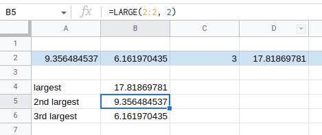
Mmmmm, I'm thinking now you are having the problem communicating, not me. :)
Let me ask again, you want to know the formulas I'm using?
 
First go vertically instead of horizontal. Use another column each for just trough and just peak. Calculate how you like. Finding the first and second value becomes easy.
 
First go vertically instead of horizontal. Use another column each for just trough and just peak. Calculate how you like. Finding the first and second value becomes easy.
I'll mull over that suggestion, thanks.
 
Mmmmm, I'm thinking now you are having the problem communicating, not me. :)
Let me ask again, you want to know the formulas I'm using?
No. I suppose it is proprietary but I've got my own.

I was just trying to help with excel formula writing if only ...

Have a good one, shutting down for the night.
 
No. I suppose it is proprietary but I've got my own.
I was just trying to help with excel formula writing if only ...
Have a good one, shutting down for the night.
No it's not proprietary, no big deal, I thought I was answering your queries, maybe someone else on ET could enlighten me what more info Suntrader requires. If formulas, please stop mincing words and just say so. :)
shutting down for the night.
Same here for the day, gotta have breakfast and also got chores to do next few hours.
 
Last edited:
Ok, will try my best at explaining.
Basic info, price moves in waves which are random in interval and height & depth.
View attachment 297404

I'm attempting to measure these waves on a spreadsheet on multiple stocks, so on a spreadsheet you'll gets peaks and troughs, once identified dotted all over the spreadsheet, they are all waving and cresting at different intervals.

Old data is on LHS of spreadsheet, new data travelling toward the RHS.
So far this morning, in the wee small hours, I have identified the Peaks and values, I've got thus far.

View attachment 297405
This is how my trial spreadsheet last panel (just working on Peaks atm) is looking so far until last close.
As you will note, it's a large spreadsheet for 16 stocks I'm dummy trialling, I've arrived at column ~148 rows of data to achieve so fars results.
I've checked the data and I'm getting accurate results on Peak dates and Peak heights.

I'll just concentrate on Peaks atm, to attempt to simplify the process, the Troughs will be a straight forward inverse copy of formulas, so I'll leave that aside in the meantime.

The next hurdle to overcome is create a table whereby Peaks are tabulated in a tidy little box showing just the stock codes and Peak values so that I can ascertain whether Peaks are rising or falling.

Row #1 is Transaction dates
Row #2 is column numbers, not part of the formulas.
The "*" are obviously formulas where there is no Peak identified.

Use the RANK function to number your peaks and troughs, then use the date as the operator. If date of MAX > date of MAX-1, then Peaks are rising

As mentioned by others, there may be a more elegant solution using VBA or Python, and remember that with Excel there are usually many ways to skin a cat. Other ways may be no more right or wrong; choose whichever you are most comfortable with.
 
I would do this in vba. The calculations will be tedious with worksheet functions as each function will be a recursion of an previous on.

it’s exactly the problem I had in college.
 
Thanks guys for the info.
I'm actually using google sheets in a chromebook, now sheets and excel have a lot in common, same math functions but not 100%.
As well Sheets don't have VBA, they use some other method.
From my experience Excel is better than Sheets, as well, the chromebooks lack some keyboard features which is pretty annoying, eg, no F2 key, no Delete key, gawd only knows why that hairbrained idea. Another thing, using public wifi is impossible on chromebook, they do that for security I believe.
But I use chromebooks as it has other advantages and MS Windows gives me the shits.

Anyhow, an update on today, got the formula function to work promptly first thing this morning to access the last value in the Rows but getting the 2nd to last value, struggled all day to suss that, so finally via using vertical data in columns rather than Rows, got a function to work for the 2nd to last values.
So, will mull over this for a short while, I may (pretty certain I will) convert all my data into columns rather than Rows as minmike mentioned a page or two back being the better method. Yeah, so most of the day bogged down on that 2nd to last value formula.
What was tripping it up were the asterisks, if I replaced them with zeros or blank cells, still the formula would read the 2nd to last asterisk, or zero, and blank cells made it worse.
Tried every trick in my book, columns data was the only way I could get a function to read correct cells.
 
Last edited:
=LARGE() and =SMALL() will give the nth largest/smallest in a series
large.png


You just need to have nothing else in the row or column that is basically representing the array/series. Then the only thing you would have to figure out is how you are appending values to that row or column.

I would figure out one symbol and then make a new sheet in the workbook for each symbol. Then make a sheet that is basically a dashboard for all the sheets for however you want to visualize the data.

VBA to me is never an option. If you need VBA then it is way easier to install conda and learn to use pandas in a jupyter notebook. Pandas came about from Wes McKinney working with trading data at AQR so it pretty much does anything you could ever want to do with trading data.

https://saturncloud.io/ is nice if you don't want to install locally and just use a cloud based jupyter notebook.
 
Back
Top